Apache Arrow vs. Parquet and ORC: Do we really need a third Apache project for columnar data representation?

Apache Parquet and Apache ORC have become a popular file formats for storing data in the Hadoop ecosystem. Their primary value proposition revolves around their “columnar data representation format”. To quickly explain what this means: many people model their data in a set of two dimensional tables where each row corresponds to an entity, and each column an attribute about that entity. However, storage is one-dimensional --- you can only read data sequentially from memory or disk in one dimension. Therefore, there are two primary options for storing tables on storage: Store one row sequentially, followed by the next row, and then the next one, etc; or store the first column sequentially, followed by the next column, and then the next one, etc.

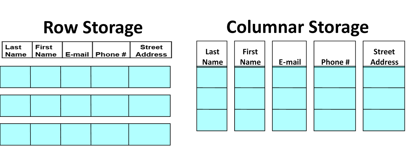
Storage layout difference between row- and column-oriented formats

For decades, the vast majority of data engines used row-oriented storage formats. This is because many early data application workloads revolved around reading, writing, and updating single entities at a time. If you store data using a columnar format and you want to extract all attributes for a particular entity, the system must jump around, finding the data for that entity from each of the separately-stored attributes. This results in a random access pattern, which results in slower access times than sequential access patterns. Therefore, columnar storage formats are a poor fit for workloads that tend to read and write entire entities at once, such as OLTP (transactional) workloads. Over time, workloads became more complex, and data analytics workloads emerged that tended to focus on only a few attributes at once; scanning through large quantities of entities to aggregate and/or process values of these attributes. Thus, storing data in a columnar fashion became more viable, and columnar formats resulted in sequential, high performance access patterns for these workloads.

Apache Arrow has recently been released with seemingly an identical value proposition as Apache Parquet and Apache ORC: it is a columnar data representation format that accelerates data analytics workloads. Yes, it is true that Parquet and ORC are designed to be used for storage on disk and Arrow is designed to be used for storage in memory. But disk and memory share the fundamental similarity that sequential access is faster than random access, and therefore the analytics workloads which tend to scan through attributes of data will perform more optimally if data is stored in columnar format no matter where data is stored --- in memory or on disk.  And if that’s the case, the workloads for which Parquet and ORC are a good fit will be the identical set of workloads for which Arrow is a good fit. If so, why do we need two different Apache projects?

Before we answer this question, let us run a simple experiment to validate the claimed advantages of column-stores. On an Amazon EC2 t2.medium instance, I created a table with 60,000,000 rows (entities) in main memory. Each row contained six attributes (columns), all of them 32-bit integers. Each row is therefore 24 bytes, and the entire table is almost 1.5GB. I created both row-oriented and column-oriented versions of this table, where the row-oriented version stores the first 24-byte row, followed by the next one, etc; and the column-oriented version stores the entire first column, followed by the next one, etc. I then ran a simple query ideally suited for column-stores --- I simply search the entire first column for a particular value. The column-oriented version of my table should therefore have to scan though just the first column and will never need to access the other five columns. Therefore it will need to scan through 60,000,000 values * 4 bytes per value = almost 0.25GB. Meanwhile the row-store will need to scan through the entire 1.5GB table because the granularity with which data can be passed from memory to the CPU (a cache line) is larger than the 24-byte tuple. Therefore, it is impossible to read just the relevant first attribute from memory without reading the other five attributes as well. So if the column-store has to read 0.25GB of data and the row-store has to read 1.5GB of data, you might expect the column-store to be 6 times faster than the row-store. However, the actual results are presented in the table below:

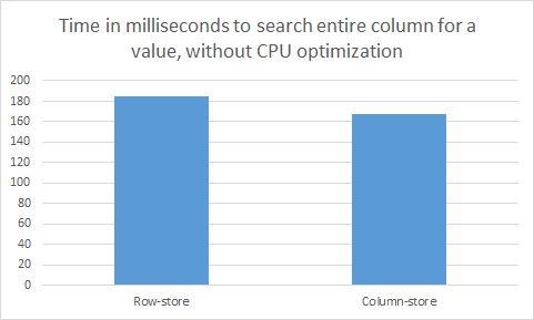
Surprisingly, the row-store and the column-store perform almost identically, despite the query being ideally suited for a column-store. The reason why this is the case is that I turned off all CPU optimizations (such as vectorization / SIMD processing) for this query. This resulted in the query being bottlenecked by CPU processing, despite the tiny amount of CPU work that has to happen for this query (just a simple integer comparison operation per row). To understand how it is possible for such a simple query to be bottlenecked by the CPU, we need to understand some basic performance specifications of typical machines. As a rough rule of thumb, sequential scans through memory can feed data from memory to the CPU at a rate of around 30GB a second. However, a modern CPU processor runs at approximately 3 GHz --- in other words they can process around 3 billion instructions a second. So even if the processor is doing a 4-byte integer comparison every single cycle, it is processing no more than 12GB a second --- a far smaller rate than the 30GB a second of data that can be sent to it. Therefore, CPU is the bottleneck, and it does not matter that the column-store only needs to send one sixth of the data from memory to the CPU relative to a row-store.

On the other hand, if I turn on CPU optimizations (by adding the ‘-O3’ compiler flag), the equation is very different. Most notably, the compiler can vectorize simple operations such as the comparison operation from our query. What this means is that originally each of the 60,000,000 integer comparisons that are required for this query happened sequentially --- each one occurring in a separate instruction from the previous. However, once vectorization is turned on, most processors can actually take four (or more) contiguous elements of our column, and do the comparison operation for all four of these elements in parallel --- in a single instruction. This effectively makes the CPU go 4 times faster (or more if it can do more than 4 elements in parallel). However, this vectorization optimization only works if each of the four elements fit in the processor register at once, which roughly means that they have to be contiguous in memory. Therefore, the column-store is able to take advantage of vectorization, while the row-store is not. Thus, when I run the same query with CPU optimizations turned on, I get the following result:

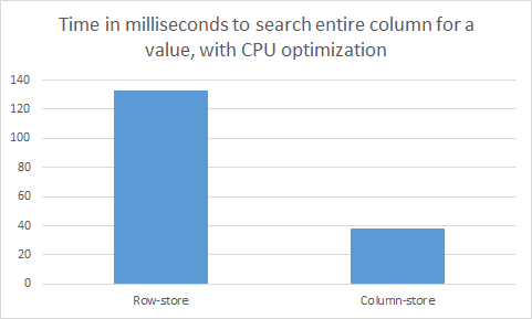
As can be seen, the EC2 processor appears to be vectorising 4 values per instruction, and therefore the column-store is 4 times faster than the row-store. However, the CPU still appears to be the bottleneck (if memory was the bottleneck, we would expect the column-store to be 6 times faster than the row-store).

We can thus conclude from this experiment that column-stores are still better than row-stores for attribute-limited, sequential scan queries like the one in our example and similar queries typically found in data analytics workloads. So indeed, it does not matter whether the data is stored on disk or in memory --- column-stores are a win for these types of workloads. However, the reason is totally different. When the table is stored on disk, the CPU is much faster than the bandwidth with which data can be transferred from disk to the CPU. Therefore, column-stores are a win because they require less data to be transferred for these workloads. On the other hand, when the table is stored in memory, the amount of data that needs to be transferred is less relevant. Instead, column-stores are a win because they are better suited to vectorized processing.  

The reason why it is so important to understand the difference in bottleneck (even though the bottom line is the same) is that certain decisions for how to organize data into storage formats will look different depending on the bottleneck. Most notably, compression decisions will look very different. In particular, for data stored on disk, where the bandwidth of getting data from disk to CPU is the bottleneck, compression is almost always a good idea. When you compress data, the total size of the data is decreased, and therefore less data needs to be transferred. However, you may have to pay additional CPU processing costs to do the decompression upon arrival. But if CPU is not the bottleneck, this is a great tradeoff to make. On the other hand, if CPU is the bottleneck, such as our experiments above where the data was located in main memory, the additional CPU cost of decompression is only going to slow down the query.

Now we can understand some of the key differences between Apache Parquet/ORC and Apache Arrow. Parquet and ORC, since they are designed for disk-resident data, support high-ratio compression algorithms such as snappy (both), gzip (Parquet), and zlib (ORC) all of which typically require decompression before data processing (and the associated CPU costs). Meanwhile, Arrow, which is designed for memory-resident-data, does not support these algorithms. The only compression currently supported by Arrow is dictionary compression, a scheme that usually does not require decompression before data processing. For example, if you want to find a particular value in a data set, you can simply search for the associated dictionary-encoded value instead. I assume that the Arrow developers will eventually read my 2006 paper on compression in column-stores and expand their compression options to include other schemes which can be operated on directly (such as run-length-encoding and bit-vector compression). I also expect that they will read the X100 compression paper which includes schemes which can be decompressed using vectorized processing. Thus, I expect that Arrow will eventually support an expanded set of compression options beyond just dictionary compression. But it is far less likely that we will see heavier-weight schemes like gzip and snappy in the Apache Arrow library any time soon.

Another difference between optimizing for main memory and optimizing for disk is that the relative difference between random reads and sequential reads is much smaller for memory than for disk. For magnetic disk, a sequential read can be 2-3 orders of magnitude faster than a random read. However, for memory, the difference is usually less than an order of magnitude. In other words, it might take hundreds or even thousands of sequential reads on disk in order to amortize the cost of the original random read to get to the beginning of the sequence. But for main memory, it takes less than ten sequential reads to amortize the cost of the original random read. This enables the batch size of Apache Arrow data to be much smaller than batch sizes of disk-oriented storage formats. Apache Arrow actually fixes batches to be no more 64K records.

So to return back to the original question: do we really need a third column-store Apache project? I would say that there are fundamental differences between main-memory column-stores and disk-resident column-stores. Main-memory column-stores, like Arrow, need to be CPU optimized and focused on vectorized processing (Arrow aligns data to 64-byte boundaries for this reason) and low-overhead compression algorithms. Disk-resident column-stores need to be focused transfer-bandwidth and support higher-compression ratio algorithms. Therefore, it makes sense to keep Arrow and Parquet/ORC as separate projects, while also continuing to maintain tight integration.

Hazelcast and the Mythical PA/EC System

(Editor’s note: I was unaware that Kyle Kingsbury was doing a linearizability analysis of Hazelcast when I was writing this post. Kyle’s analysis resulted in Greg Luck, Hazelcast’s CEO, to write a blog post where he cited the PACELC theorem, and came to some of the same conclusions that I came to in writing this post. This post, however, was 98% written before both Kyle’s and Greg’s posts, but their posts got me to accelerate the completion of my analysis and publish it now.)

Seven years ago, I introduced the PACELC theorem as a mechanism to more clearly explain the consistency tradeoffs in building distributed systems. At that time, many people were familiar with the consistency vs. availability trade-off that was made well-known by the CAP theorem. However, it was common amongst people unfamiliar with the details of CAP theorem to believe that this tradeoff is always present in a distributed system. However, the truth is that the CAP consistency-availability tradeoff actually describes a very rare corner case. Only when there is an actual network partition --- an increasingly unusual event in modern day infrastructures ---  does the consistency-availability tradeoff present itself. At all other times, it is possible to be both available and consistent. Nonetheless, many systems choose not to be fully consistent at all times. The reason for this has nothing to do with the CAP tradeoff. Instead, there is a separate latency vs. consistency tradeoff. Enforcing consistency requires either (1) synchronization messages between machines that must remain consistent with each other or (2) all requests involving a particular data item to be served by a single master for that data item instead of the closest replica to the location where the request originates. Both of these options come with a latency cost. By relaxing consistency and serving reads and writes directly from a closest replica (without synchronization with other replicas), latency can be improved --- sometimes by an order of magnitude.

Therefore, I felt that it was important to clearly tease apart these separate consistency tradeoffs. This led to the PACELC theorem: if there is a partition (P), how does the system trade off availability and consistency (A and C); else (E), when the system is running normally in the absence of partitions, how does the system trade off latency (L) and consistency (C)?

In general, the PACELC theorem leads to four categories of systems: PC/EC, PA/EL, PC/EL, and PA/EC. However, in practice, an application will either go to the effort of building on top of a reduced consistency system or it will not. If it goes to this effort, it stands to benefit in two areas: availability upon a partition, and latency in everyday operation. It is unusual for a system to go to this effort and choose only to attain benefit in one area. Hence, two of these four categories are more common than the other two: PC/EC systems designed for applications that can never sacrifice consistency, and PA/EL systems that are designed for applications that are capable of being built over a reduced consistency system. Despite being less common, PACELC nonetheless theorizes about the existence of PC/EL and PA/EC systems. At the time when I originally introduced PACELC, I gave the example of PNUTS as a PC/EL system. However, I could not think of any good examples of PA/EC systems. Even in my extended article on PACELC in the CAP-anniversary edition of IEEE Computer, I only gave a somewhat hand-wavey example of a PA/EC system.

The basic problem with PA/EC systems is the following: although partitions are a rare event, they are not impossible. Any application built on top of a PA system must have mechanisms in place to deal with inconsistencies that arise during these partition events. But once they have these mechanisms in place, why not benefit during normal operation and get better latency as well?

Over the past few weeks, I have been looking more deeply at the In-Memory Data Grid (“IMDG”) market, and took an especially deep dive into Hazelcast, a ubiquitous open source implementation of a IMDG, with hundreds of thousands of in production deployments. It turns out that Hazelcast (and, indeed, most of the in-memory data grid industry) is a real implementation of the mythical PA/EC system.

In order to understand why PA/EC makes sense for Hazelcast and other IMDGs, we need to first discuss some background material on (1) Hazelcast use cases, (2) data replication and (3) PACELC.

Hazelcast use cases

The most common use case for Hazelcast is the following. Let’s say that you write a Java program that stores and manipulates data inside popular Java collections and data structures, e.g., Queue, Map, AtomicLong, or Multimap. You may want to run this program in multiple different clients, all accessing the same Java collections and data structures. Furthermore, these data structures may get so large that they cannot fit in memory on a single server. Hazelcast comes to the rescue --- it provides a distributed implementation of these Java data structures, thereby enabling scalable utilization of them. Users interact with Hazelcast the same way that they interacted with their local data structures, but behind the scenes, Hazelcast is distributing and replicating them across a cluster of machines.

The vast majority of Hazelcast use cases are within a single computing cluster. Both the client programs and the Hazelcast data structures are located in the same physical region.

Data replication

In general, any arbitrary system may choose to replicate data for one of two primary reasons: Either they want to improve fault tolerance (if a server containing some of the data fails, a replica server can be accessed instead), or they want to improve request latency (messages that have to travel farther distances take longer to transmit; therefore, having a replica of the data “near” locations from which they are typically accessed can improve request latency).

As mentioned above, in-memory data grids are typically running in the same region as the clients which access them. Therefore, only the first reason to replicate data (fault tolerance) applies. (This reason alone is enough to justify the costs of replication in any scalable system. The more physical machines that exist in the system, the more likely it is that at least one machine will fail at any given point in time. Therefore, the bigger the system, the more you need to replicate for fault tolerance).

If the replicas only exist for fault tolerance and not for performance, there is no fundamental requirement to ever access them except in the case of a failure. All reads and writes can be directed to the primary copy of any data item, with the replicas only ever accessed if the primary is not available. (In such a scenario, it is a good idea to mix primary and replica partitions on servers across the cluster, in order to prevent underutilization of server resources.) If all reads and writes go to the same location, this leads to 100% consistency and linearizability (in the absence of failures) since it is easy for a single server to ensure that reads reflect the most recent writes.

What this means for PACELC

Recall what I wrote above about the latency vs. consistency tradeoff: “Enforcing consistency requires either (1) synchronization messages between machines that must remain consistent with each other or (2) all requests involving a particular data item to be served by a single master for that data item instead of the closest replica to the location where the request originates. Both of these options come with a latency cost.” In truth, option (2) does not come with a latency cost when all requests originate from a location closest to the master replica. It’s only when messages travel for longer than the distance to the nearest replica where a cost materializes. In order words, there is no consistency vs. latency tradeoff in the typical Hazelcast use case.

Thus, we should clarify at this point that the PACELC theorem assumes that requests may originate from any arbitrary location. The ELC part of PACELC disappears if all requests come from the same location. I would argue that the CAP theorem makes the same assumption, but such an argument is not as straightforward, and requires a refined discussion about the CAP theorem which is outside scope of this particular blog post.

Failures and partitions

Up until now, we have said that as long as the master node does not fail, if it serves all reads and writes, then full consistency is achieved. The obvious next question is: what happens if the master node fails and a new master takes over? In such a scenario, the ability of the system to maintain consistency depends on how replication is performed. If replication was asynchronous, then consistency cannot be guaranteed, since some updates may have been performed on the old master, but had not yet been replicated to the new master before the old master failed. If all data had been synchronously replicated to the new master, then full consistency can still be guaranteed.

A failed node is logically equivalent to a partition where the failed node is located in one partition and every other node is in the other partition, and all client requests can reach the second partition but not the first. If the failed node is the master node, and replication was asynchronous, then both the CAP theorem and the PAC part of PACELC state that there are only two choices: quiesce the entire system since the only consistent copy is not accessible (i.e. choosing consistency over availability), or serve reads and writes from nodes in the available partition (i.e. choosing availability over consistency).  

Hazelcast by default uses “synchronous” replication, which is actually an interesting hybrid between asynchronous and synchronous replication. The master asynchronously sends the writes to the replicas, and each replica acknowledges these writes to the client. The client synchronously waits for these acknowledgments before returning from the call. However, if the requisite number of acknowledgments do not arrive before the end of a time out period, the call either returns with the write succeeding or throws an exception, depending on configuration. If Hazelcast had been configured to throw an exception, the client can retry the operation.  Hazelcast also has an anti-entropy algorithm that works offline to re-synchronize replicas with the master to repair missed replications. However, either way --- until the point where the missed replication has been repaired either through the anti-entropy algorithm or through a client retry, the system is temporarily in a state where the write has succeeded on the master but not on at least one replica.

In addition to the hybrid synchronous algorithm described above, Hazelcast also can be configured to use standard asynchronous replication. When configured in this way, the client does not wait for acknowledgments from the replicas before returning from the call. Thus, updates that failed to get replicated will go undetected until the anti-entropy algorithm identifies and repairs the missed replication.  

Thus, either way --- whether Hazelcast is configured to use standard asynchronous replication or to use the default hybrid “synchronous” model --- it is possible for the write call to return with the write only succeeding on the master.

If the master node fails, Hazelcast selects a new master to serve reads and writes, even though (as we just mentioned) it is possible that the new master does not have all the writes from the original master. If there is a network partition, the original master will remain the master for its partition, but the other partition will select its own master. Again, this second master may not have all the writes from the original master. Furthermore, a full split brain situation may occur, where the masters for the two different partitions independently accept writes to their partition, thereby causing the partitions to diverge further. However, Hazelcast does have a “split brain protection” feature that prevents significant divergence. The way this feature works is that the system can be configured to define a minimum size for read and write operations. If this minimum size is set to be larger than half of the size of the cluster, then the smaller partition will not accept reads and writes, which prevents further divergence from the larger partition. However, it can take 10s of seconds for the smaller partition to realize how small it is (although Hazelcast claims it will be much faster than this in 3.9.1 and 3.10). Thus there is a delay before the split brain protection kicks in, and the partitions can diverge during this delay period.

The bottom line here is that both if the master fails and also in the (rare) case of a network partition, a new master is selected that may not have all the updates from the original master. The system always remains available, but the second master is allowed to temporarily diverge from the original master. Thus, Hazelcast is PA/EC in PACELC. If the master has failed or partitioned, Hazelcast choses availability over consistency. However, in the absence of failures or partitions, Hazelcast is fully consistent. (As mentioned above, Hazelcast also achieves low latency in the absence of failures or partitions in their primary use case. However, it is appropriate to label Hazelcast EC rather than EL since if a request were to theoretically originate in a location that is far from the master, it would still choose consistency over latency and serve the request from the master.)

Indeed, any system that that serves reads and writes from the master, but elects a new master upon a failure, where this new master is not 100% guaranteed to have seen all of the writes from the original master, will be PA/EC in PACELC. So the PA/EC category is larger than I originally had expected.

I would still argue, however, that PA/EC systems are fundamentally confusing to the end user. If the system cannot guarantee consistency in all cases, then the end user is forced to handle cases of inconsistency in application logic. And once they have the code written to handle these cases (e.g., by including merge functions that resolve situations where replicas may diverge), then the value of the system being consistent in the absence of failures or partitions is significantly reduced. PA/EC systems thus only make sense for applications for which availability takes priority over consistency, but where the code that handles inconsistencies needs to be run as infrequently as possible --- e.g. when the code involves a real world charge (such as refunding a customer’s account) or significant performance costs.

Since not all applications fit into the above category, I suspect that many PA/EC systems will have settings to either increase consistency in order to become fully consistent (i.e. become PC instead of PA) or reduce consistency guarantees in the “else case” (i.e., become EL instead of EC).

Indeed, Hazelcast is such a system and can be configured to be EL rather than EC. There are several ways to accomplish this, but the primary mechanism is through their Near Cache feature. Near Cache is a client side cache of recently accessed data items. If the data items stored in the Near Cache are updated by a different client, these changes are not synchronously replicated to the first client’s Near Cache. Hence, the Near Cache is not kept consistent with the master version of the data (instead it is “eventually consistent”). However, reads by the client are served by its Near Cache if a copy of the data item to be read is stored there. Therefore, excellent latency (less than one microsecond) can be achieved at the cost of consistency --- EL in PACELC.

Furthermore, Hazelcast also supports replication of clusters over a WAN. For example, in a disaster recovery use case, all writes go to the primary cluster, and they are asynchronously replicated to a backup cluster. Alternatively, both clusters can accept writes, and they are asynchronously replicated to the other cluster (the application is responsible for resolving conflicts of conflicting writes to the different clusters using a conflict resolution strategy registered with Hazelcast). Unlike what we discussed earlier, in this case read requests may originate from arbitrary locations rather than always from a location near the master. Hazelcast serves these reads from the closest location, even though it may not have the most up to date copy of the data. Thus, Hazelcast is EL by default for WAN replication.  

In summary, through my investigation of Hazelcast (and in-memory data grids in general), I have discovered a new category of PA/EC systems. However, due to the confusing nature of PA/EC systems, it is no surprise that Hazelcast can be configured to be PA/EL in addition to its PA/EC default.